Listening to Caltrain: Analyzing Train Whistles with Data Science
August 29th, 2014
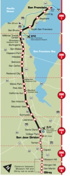 Many people who live and work in Silicon Valley depend on Caltrain for transportation. And because the SVDS headquarters are in Sunnyvale, not far from a station, Caltrain is literally in our own backyard. So, as an R&D project, we have been playing with data science techniques to understand and predict delays in the Caltrain system.
A recent talk at Hadoop Summit explains our approach and why we’re doing this. Ultimately we will offer a mobile app for Caltrain riders, which will provide both schedule information and real-time predictions of arrivals based on system delays. You might think this would be easy, since Caltrain provides schedules and even a real-time API. But as with all trains, Caltrain sometimes gets behind schedule. Sometimes its API estimates are off. Other times its API crashes and provides no information. So we’ve been attempting to get a larger view of the Caltrain system from a variety of sources.
We want to apply data science to a variety of local, distributed, redundant, and possibly unreliable information sources in order to understand the state of the system. Data sources are never completely reliable and consistent across a large system, so this gives us experience producing predictions from messy and possibly erroneous data.
Our first task is to detect and identify trains as they pass our office. For this purpose, we’ve set up audio and video feeds that regularly record and analyze signals.
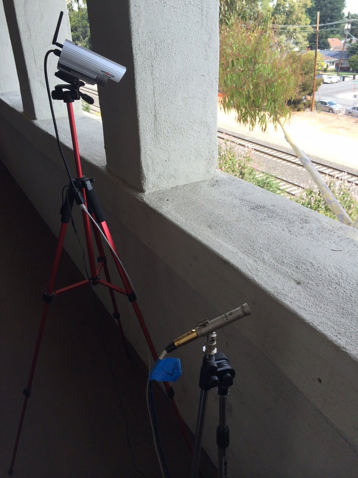
We set up audio and video capture on our office porch, right next to the tracks.
We’d like to extract as much information as possible from these sources. Understanding the direction and speed of each train allows us to determine whether we observed a local or express train—and ultimately which scheduled run number it was and whether it was early, on time, or late.
The way we approach complex problems like this at SVDS is to break it down into smaller problems and iterate to the ultimate solution. We began focused on the audio stream, and pursued an agile approach to developing our ability to use that signal to provide the information we needed to understand what trains were passing by our office.
Obtaining the Signal
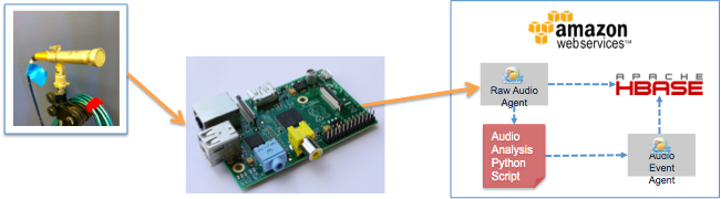
Our audio setup consists of a microphone on a stand (shown below) with an omnidirectional capsule, which “listens” in all directions. The microphone is connected to a pre-amp that amplifies the signal to a usable level, and converts the analog signal to a digital representation we can process. We feed the digital signals into a Raspberry Pi board, where we use PyAudio to serialize the audio into an array of 2-byte integers. The sound data plus metadata is then passed to Flume on AWS. (A presentation at OSCON 2014 describes this work in more detail).
Signal Processing
The first question we want to answer with our audio data is: was this a local or an express train? Local trains stop at the local Sunnyvale station whereas express trains (with few exceptions) pass through without stopping. Can we tell the difference from the sound?
The sound clips from our microphones sound fairly different to human ears, so you might think it’s easy to tell them apart automatically. However, as with most real-world problems, there are complications. We are near an intersection so there is road noise (honking horns, car engines, squealing brakes, and so on) that the microphone picks up. For this reason, we’ve tuned the audio system to extract only the train “whistles” (horn blasts, really), which you can hear in the sound clips above. The fundamental frequencies of these whistles are around 300-400 Hz. These come into our dataset as dominant frequency clips, which look like this:
|
Timestamp |
Date and time |
Audio sequence |
|
1400880301 |
2014-05-23 14:25:01 |
345, 342, 327 |
|
1400890826 |
2014-05-23 17:20:26 |
344, 343, 344, 339, 337, 334, 331, 330, 330, 329, 329, 327, 326, 327, 326 |
|
1400894242 |
2014-05-23 18:17:22 |
343, 346, 327, 326, 326 |
|
1401240295 |
2014-05-27 18:24:55 |
338, 337, 333, 332, 331, 330, 329, 328, 327, 327, 327 |
|
1401284409 |
2014-05-28 06:40:09 |
338, 337, 336, 336, 336, 325, 320, 319, 319, 319, 319 |
Each row represents the sounds of one train passing. Each number in the audio sequence column is a fundamental frequency of an audio timeslice (so longer sequences represent longer whistles). We want to classify each train/row as local or express. This is where it becomes a data science problem. We have hand-labeled some of this data reliably, so it looks like it could be a standard two-class classification problem. However, our data comprises sequences of differing lengths.
Hidden Markov Model
A method that can be useful for analyzing sequences in general—and audio tones in particular—is called a Hidden Markov Model (HMM). Hidden Markov Models have been around for decades and they are commonly used for labeling sequences. They have been called the “Legos of computational sequence analysis.” They are an important part of the speech recognition technology underlying Apple’s Siri and Microsoft’s Cortana personal assistants, where they are used to judge probabilities of sequences and to label their parts. They’re also very common in computational biology for labeling gene sequences.
Unfortunately, for our purposes HMMs have several drawbacks. They tend to require a lot of processing resources to develop, and they can be unstable. Most importantly, consider our task: we simply want to discriminate between two signals—an express train and a local train. If we can reframe the problem and reduce the sequence to a set of features, we will have many additional data science methods we can use to do this without some of the drawbacks of HMMs.
Other Models
Following a principle of using the simplest techniques first, we chose two basic classification techniques: a decision tree and logistic regression. Both methods try to separate instances of the two classes. Conceptually, a decision tree tries to “chop up” the space with vertical and horizontal slices. It does this by choosing one variable at a time to threshold and building a tree of the variables. Logistic regression tries to put a single plane through the space to separate the two. Which works better for a given task depends on the data.
First, we have to decide on a data representation. Since our data is a set of sequences, it’s not as simple as providing the raw data; we have to provide summary statistics of each sequence. We chose these basic measures:
-
The minimum and maximum value (wmin and wmax) of each sequence.
-
The average frequency value (wavg).
-
The length of the sequence (wlen).
-
The span of frequencies (wspan), which is the maximum minus the minimum.
So what did the methods learn? The decision tree learned was simple and compact, and used only two variables. Here is the printed representation of the tree:
wmin <= 315
| wmin <= 305: l (3.0/1.0)
| wmin > 305: e (15.0/1.0)
wmin > 315
| wspan <= 8.333333: l (131.0/1.0)
| wspan > 8.333333
| | wmin <= 326: l (5.0)
| | wmin > 326: e (6.0)
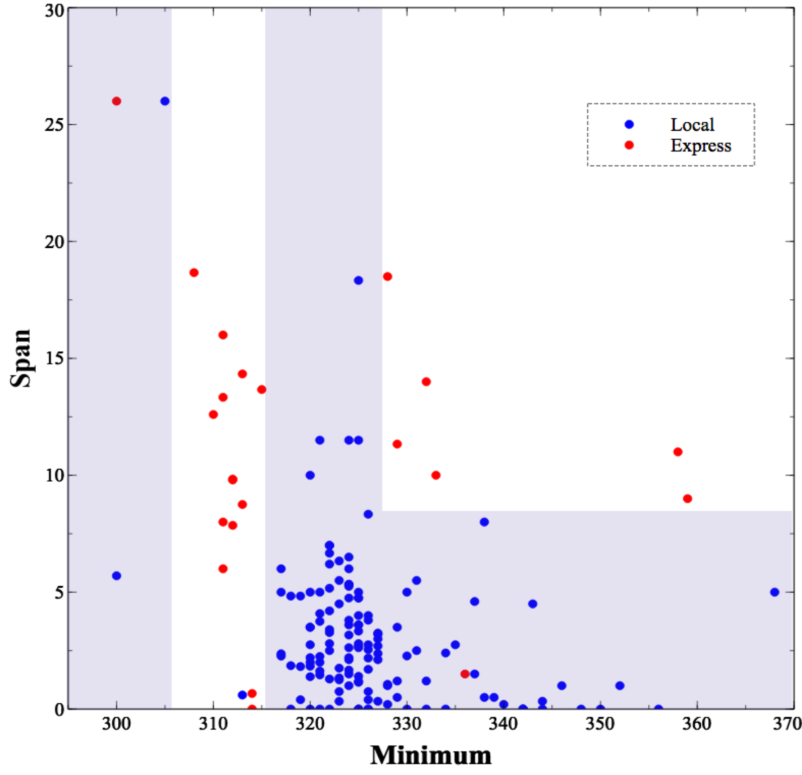 This is technically accurate, but not very informative. The upper graph is a more informative view of the tree, showing how it decided to cut up the space.
The blue regions are the areas the decision tree classifies as local, and the unshaded regions are the express trains. What is this telling us? Loosely speaking, we’re seeing the effects of the Doppler effect as the trains go by. Express trains pass by without stopping, so they’re usually going pretty fast when they pass our offices. This causes a Doppler shift in their whistles: a high whistle frequency as they approach followed by a falling, lower whistle as they move away. This shift causes a higher span value as you can see in the graph, as well as a lower minimum value. The local trains, moving more slowly, have much less of a shift.
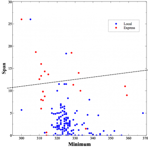 For comparison, the lower graph is the logistic regression decision surface on the same space.
Logistic regression is limited to a single surface (the dashed line, in this case) though it can have any orientation. In this case, whistles above the line are classified as express and those below the line as local. The decision tree has an advantage here, because the two instances can’t really be separated with a single line. As you can see, the logistic regression result makes a fair number of mistakes.
Which Model is Best?
The decision tree is surprisingly accurate: it’s able to classify whistles with 98% accuracy. Logistic regression only performs at about 90%.
You might conclude, based on these diagrams and performance numbers, that decision trees are somehow better than logistic regression. The two methods actually have different characteristics, and neither is uniformly better than the other. Claudia Perlich has an interesting paper comparing the two. Further, there are some problems where reframing the way the data is analyzed from a sequence of observations in time, to a set of characteristics describing a single event, may not be possible and HMMs and similar methods would be required. The important lessons here are to start simple and only take on additional complexity when necessary, and don’t assume that one technique is always going to be better than another.
When combining this analysis with the video feed, social media, and others, we can iterate each of those approaches, and integrate them to answer the larger question of “what is the current status of run 227?” Each of those signals, and the sub-questions we seek to answer with them, will require a similar iteration of technique. Is it better to determine direction using the video camera, or add a second microphone and use the difference in time of when the signal arrives at the microphone to determine direction? Stay tuned as we work our way through those questions.
Flexibility is Key
At SVDS, we find an agile approach to solving data science problems like this is critical to success precisely because of the ambiguity around what techniques and associated data transformations will prove successful in solving the problem. Our ultimate goal is to provide insight into system state that is based in part on the local/express classification problem discussed here, but is a far more complex problem.
At the onset we don’t know how successful we will be solving each of the sub-problems, nor which signals we will use to do so. We do know from experience that an ensemble of signals and approaches will provide the best chance for success, and that a battle plan which presumes to know which combination of data and technique will be successful won’t survive the first day of battle.
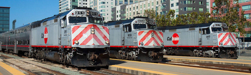
Header image by David Gubler. Used under CC BY-SA 2.0.