
The Basics of Classifier Evaluation: Part 1
August 5th, 2015
If it’s easy, it’s probably wrong.
If you’re fresh out of a data science course, or have simply been trying to pick up the basics on your own, you’ve probably attacked a few data problems. You’ve experimented with different classifiers, different feature sets, maybe different parameter sets, and so on. Eventually you’re going to think about evaluation: how well does your classifier work?
I’m assuming you already know basic evaluation methodology: you know not to test on the training set, maybe you know cross-validation, and maybe you know how to draw confidence bars or even do t-tests. That’s data science 101, and you’re probably well familiar with it by now. I’m not talking about that. What I’m talking about is something more basic, but even harder: how should you measure the performance of your classifier?
The obvious answer is to use accuracy: the number of examples it classifies correctly. You have a classifier that takes test examples and hypothesizes classes for each. On every test example, its guess is either right or wrong. You simply measure the number of correct decisions your classifier makes, divide by the total number of test examples, and the result is the accuracy of your classifier. It’s that simple. The vast majority of research results report accuracy, and many practical projects do too. It’s the default metric.
What’s wrong with this approach? Accuracy is a simplistic measure that is misleading on many real-world problems. In fact, the best way to get a painful “But it worked in the lab, why doesn’t it work in the field?” experience is to use accuracy as an evaluation metric.
What’s wrong with accuracy?
To illustrate the problems, let’s start with a simple two-class domain. Every classifier for this domain sees examples from the two classes and outputs one of two possible judgments: Y or N. Given a test set and a specific classifier, you can place each decision as:
- a positive example classified as positive. This is a true positive.
- a positive example misclassified as negative. This is a false negative.
- a negative example classified as negative. This is a true negative.
- a negative example misclassified as positive. This is a false positive.
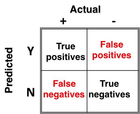
We can create a 2×2 matrix with the columns as true classes and the rows as the hypothesized classes. It looks like this:
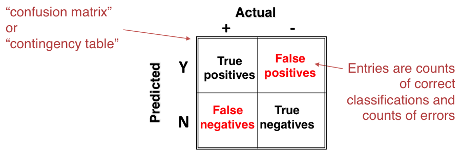
Each instance contributes to the count in exactly one of the cells. This is the way to think about your classifier.
Accuracy is simply the sum of the diagonals divided by the total:

What’s wrong with this?
The problem with class imbalance
Accuracy simply treats all examples the same and reports a percentage of correct responses. Accuracy may be fine when you’re dealing with balanced (or approximately balanced) datasets. The further you get from 50/50, the more accuracy misleads. Consider a dataset with a 99:1 split of negatives to positives. Simply guessing the majority class yields a 99% accurate classifier!
In the real world, imbalanced domains are the rule, not the exception! Outside of academia, I have never dealt with a balanced dataset. The reason is fairly straightforward. In many cases, machine learning is used to process populations consisting of a large number of negative (uninteresting) examples and a small number of positive (interesting, alarm-worthy) examples.
Examples of such domains are fraud detection (1% fraud is a huge problem; 0.1% is closer), HIV screening (prevalence in the USA is ~0.4%), predicting disk drive failures (~1% per year), click-through advertising response rates (0.09%), factory production defect rates (0.1%) — the list goes on. Imbalance is everywhere.
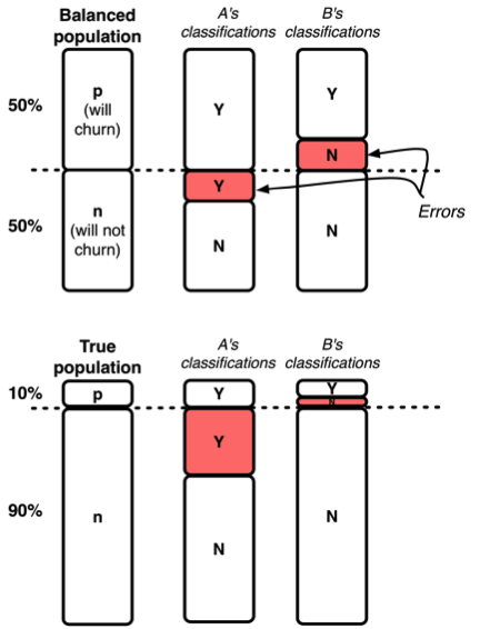 How does this complicate evaluation? An example is shown in the diagram at left. This is a churn problem—we want to recognize which customers are likely to churn (cancel their contracts) soon.
The top half shows the training population. We’ve balanced the population so half is positive, half is negative. We’ve trained two classifiers, A and B. They each make the same percentage of errors, so in this particular dataset their accuracies are identical, as shown by the red areas in the top half.
The bottom half shows the same two classifiers in a testing environment, where the population is now 10% (will churn) to 90% (will not churn). This is far more realistic. Notice that A is now far worse because its errors are false positives.
There are two lessons from this example. One is that you should know more about your classifiers than what accuracy tells you. The other is that, regardless of what population you train on, you should always test on thereal population—the one you care about.
The problem with error costs
There is a second problem. Consider the domain of predicting click-through advertising responses. The expected rate (the class prior) of click-throughs is about 0.09%. This means that a classifier that unconditionally says, “No, the user won’t click” has an accuracy of 99.91%. What’s wrong with this? Strictly speaking, nothing! That’s great performance—if accuracy was what you cared about.
The problem is that you care about some classes much more than others. In this case, you care far more about those 0.09% of people who click through than the 99.91% who don’t. To put it more precisely, you care about which error you make: showing an ad to a few people who won’t click on it (a False Positive in the matrix above) isn’t so bad, but failing to show an ad to people who would click on it (a False Negative) is far worse. Targeting the right people for the ad is, after all, the whole reason you’re building a classifier in the first place.
Different error costs are common in many domains. In medical diagnosis, the cost of diagnosing cancer when it doesn’t exist is different from missing a genuine case. In document classification, the cost of retrieving an irrelevant document is different from the cost of missing an interesting one, and so on.
What about public data sets?
If you’ve worked with databases from somewhere like the UCI Dataset Repository, you may have noticed that they don’t seem to have these issues. The classes are usually fairly balanced, and when error cost information is provided, it seems to be exact and unproblematic. While these datasets may have originated from real problems, in many cases they have been cleaned up, artificially balanced, and provided with precise error costs. Kaggle competitions have similar issues—contest organizers must be able to judge submissions and declare a clear winner, so the evaluation criteria are carefully laid out in advance.
Other evaluation metrics
By this point, you’ve hopefully become convinced that plain classification accuracy is a poor metric for real-world domains. What should you use instead? Many other evaluation metrics have been developed. It is important to remember that each is simply a different way of summarizing the confusion matrix.
Here are some metrics you’ll likely come across:
- true positive rate = TP/(TP+FN) = 1 − false negative rate
- false positive rate = FP/(FP+TN) = 1 − true negative rate
- sensitivity = true positive rate
- specificity = true negative rate
- positive predictive value = TP/(TP+FP)
- recall = TP / (TP+FN) = true positive rate
- precision = TP / (TP+FP)
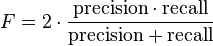
- F-score is the harmonic mean of precision and recall:
- G-score is the geometric mean of precision and recall:
Two other measures are worth mentioning, though their exact definitions are too elaborate to explain here. Cohen’s Kappa is a measure of agreement that takes into account how much agreement could be expected by chance. It does this by taking into account the class imbalance and the classifier’s tendency to vote Yes or No. The Mann-Whitney U test is a general measure of separation ability of the classifier. It measures how well the classifier can rank positive instances above negative instances.
Expected cost
Given all of these numbers, which is the right one to measure? We’ll avoid the customary Statistics answer (“It depends”), and answer: none of the above.
The confusion matrix contains frequencies of the four different outcomes. The most precise way to solve the problem is to use these four numbers to calculate expected cost (or equivalently, expected benefit). You may recall that the standard form of an expected value is to take the probability of each situation and multiply it by its value. We convert the numbers in the matrix above, then we have to the costs and benefits for each of the four. The final calculation is the sum:
Expected cost = p(p)×cost(p) + p(n)×cost(n)
Here p(p) and p(n) are the probabilities of each class, also called the class priors. cost(p) is shorthand for the cost of dealing with a positive example. What is this? We have to break it apart into two cases: if we get it right (a true positive) and if we get it wrong (a false negative).
cost(p) = p(true positive)×benefit(true positive) + p(false negative)×cost(false negative)
Similarly for the negative class: if we get it right it’s a true negative, else it’s a false positive. Expanding out the entire expected cost equation, we get the messy (but hopefully understandable) equation:
Expected cost = p(p) × [ p(true positive) × benefit(true positive)
                        + p(false negative) × cost(false negative) ]
              + p(n) × [ p(true negative) × benefit(true negative)
                        + p(false positive) × cost(false positive) ]
This is much more precise than accuracy since it splits apart each of the four possibilities for every decision and multiplies it by the corresponding cost or benefit of that decision. The priors p(p) and p(n) you can estimate directly from your data. The four p(true positive), … expressions you get from your classifier; specifically, from the confusion matrix that comes out of a classifier on a test sample. The cost() and benefit() values are extrinsic values that can’t be derived from data. They’re quantifications of the real-world consequences of the classifier’s decisions These must be estimated based on expert knowledge of the domain.
Ideally, this is the way you should evaluate a classifier if you want to reduce its performance to a single number. When you have a set of classifiers and you want to choose the best one, this method gives you a way of precisely measuring how well each classifier will perform.
Lingering questions
If you’ve read this far, you may be thinking: “Wait, what happens if I don’t have error costs? What if they change? What if I want to see graphs of performance? Isn’t there anything I can get besides a simple point estimate? And if estimated cost is the simple answer to everything, why did scikit-learn implement dozens of different metrics? ”
All good questions. The next blog post, Part 2, will answer them.