Predictive Maintenance for IoT

March 30th, 2017

At a fundamental level, the Internet of Things (IoT) represents a set of real-world “things” networked to communicate with each other, other devices, and services over the internet. Each “thing” might be able to capture and relay data about itself or its environment, and maybe even do some limited on-board computation with that data. Many consider this the next step in the evolution of the internet: massive networks of smart devices, seamlessly integrated with the physical world.

The IoT has also drawn attention for its immense commercial value, with applications across a diverse set of industries from transportation to medical devices. As a result of the hype, these applications are often only discussed in the abstract, and the details of their implementation are usually left as an exercise to the reader. In this post, we’ll cut through some of this ambiguity and introduce an example data science problem relevant to the IoT world.

Predictive maintenance

Let’s look at a real world example of a costly issue—equipment failures. Traditionally, the strategy to address them is to conduct preventative maintenance at regular time intervals. These schedules tend to be very conservative, and are often based on expert judgement or operator experience. The result is a process that virtually guarantees higher-than-necessary maintenance costs, and can be difficult or impossible to adapt to a highly complex or changing industrial scenario.

With the careful application of data science techniques, the IoT presents an appealing alternative. When equipment is instrumented with sensors and networked to transmit this sensor data, problems can be diagnosed across the fleet in real time, and the future health of individual units can be predicted in order to enable on-demand maintenance. This strategy, known as predictive (or condition-based) maintenance, is frequently cited as one of the most promising and lucrative industrial applications of the IoT.

Exploring an example

To better illustrate predictive maintenance in practice, let’s explore an open data set that poses a related problem. The Turbofan Engine Degradation Simulation data set was released in 2008 by the Prognostics Center of Excellence at NASA’s Ames research center. It consists of sensor readings from a fleet of simulated aircraft gas turbine engines, recorded as multiple multivariate time series.

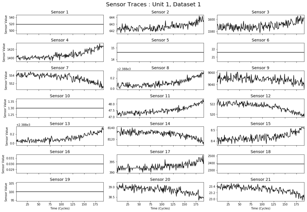
Figure showing readings from sensors on a single engine in our data set.

The figure above shows the readings from the sensors on a single engine in the data set. Each of the sensors measures something about the physical state of the engine, like the temperature of a component or the speed of a fan. Notice that some sensor channels are quite noisy and appear to increase or decrease over time, while others don’t appear to change at all. This is exactly the kind of data you might expect an industrial IoT system to produce— multivariate series of sensor measurements each with its own amount of noise, and potentially containing lots of missing or uninformative values.

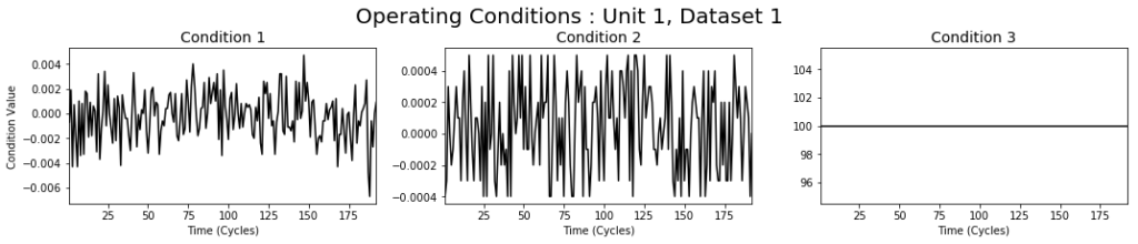
In addition to internal sensor measurements, each unit in an industrial IoT system might measure something about the outside world or the conditions in which it’s operating. In our data set, each engine operates under slightly different conditions, characterized by three dimensions which change over time (e.g. altitude or external air pressure). The figure below shows the values of these operational conditions over time for the same example engine.

Figure showing the values of operational conditions over time for the sample example engine.

The data set consists of separate training and test sets. In both, each engine starts with a different (unknown) level of wear, and is allowed to run until failure. In the training set, all of the sensor measurements are recorded at all time steps up until the moment of failure.

Figure showing all 21 sensor channels for a random sample of 10 engines from the training set, plotted against time.

The figure above shows all 21 sensor channels for a random sample of 10 engines from the training set, plotted against time. Note that each subplot contains 10 lines (one for each engine). It’s apparent from this figure that, perhaps due to their different initial conditions, each engine has a slightly different lifetime and failure pattern. This highlights the fact that each engine’s progress in time is not quite aligned with any other. This means, for instance, that we can’t directly compare the fifth cycle of one engine to the fifth cycle of another.

Exploring failure modes

Because we know when each engine in the training set will fail, we can compute a “time before failure” value at each time step, defined as an engine’s elapsed life at that time minus its total lifetime. This number is a sort of countdown to failure for each engine, and it allows us to align different engines’ data to a common end point. The figure below shows the sensor channels from the same engines as the previous figure, now plotted against their time before failure. Note that each engine now ends at the same instant (t=0), as indicated by the red line.

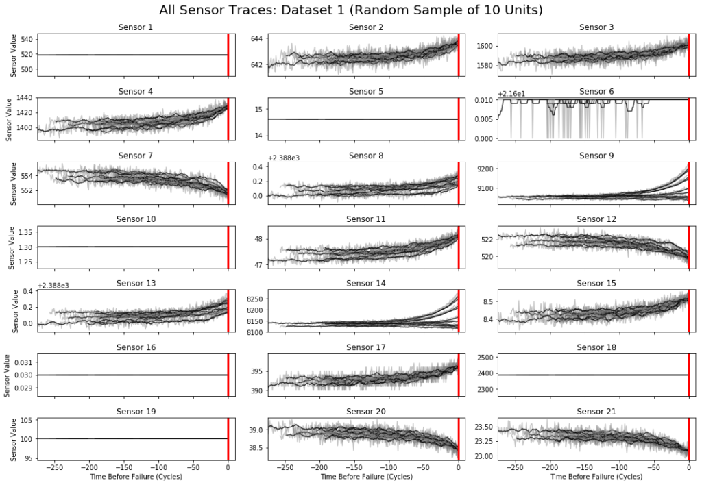
Figure showing sensor channels plotted against their time before failure.

Aligning the data in this way allows us to observe some patterns. For instance, we see that some sensor readings consistently rise or fall right before a failure, while others (e.g. sensor 14) exhibit different failure behavior across different engines. This illustrates a subtle yet important aspect of many predictive maintenance problems: failure is often a confluence of different processes, and as a result, “things” in the real world are likely to exhibit multiple failure modes.

The prediction challenge

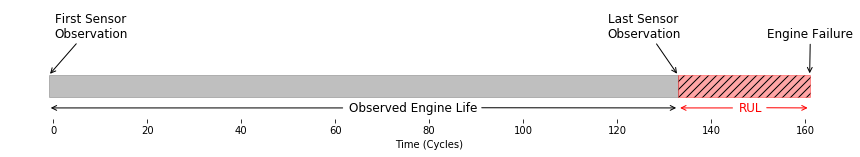
Diagram showing observed engine life

The test set is similar to the training set, except that each engine’s measurements are truncated some (unknown) amount of time before it fails. The diagram above indicates the central prediction task at hand. After observing the engine’s sensor measurements and operating conditions for some amount of time (133 cycles in the diagram), the challenge is to predict the amount of time the engine will continue to function before it fails. This number, represented by the red area in the diagram, is called the remaining useful life (RUL) of the engine. Note that for the engines in the test set, we can’t align the sensor readings to a ‘time before failure’ as we did in the section above, since now we don’t know when the engines will fail.

In essence, estimating the RUL in this way gets to the heart of the predictive maintenance problem in the IoT—we are tasked with predicting when each “thing” will fail given some information about its age, current condition, past operational history, and the recorded history of other “things” like it. In production, such a predictive model could be used for real time monitoring and alerting, and given some on-board computation, it might even enable equipment to schedule its own maintenance.

The cost of an incorrect prediction

One of the most important considerations when evaluating predictive maintenance models is the cost of an incorrect prediction. To understand why, imagine that we’ve trained a model on the data above, and are now using it in production to tell us when we should bring our airplanes in for service. If our model happens to underestimate the true RUL of a particular engine, we might bring it in for service too early when it could have operated for a bit longer without issue. What would happen if our model was to overestimate the true RUL instead? In that case, we might allow a degrading aircraft to keep flying, and risk catastrophic engine failure. Clearly, the costs of these two outcomes are not the same.

Table showing the value of cost function versus prediction error

To capture the different costs associated with different kinds of incorrect predictions, one approach is to use an asymmetric cost function for evaluation. Typically, such a function is applied to the output of a model (RUL predictions in our case) and returns the total “penalty” associated with that model’s predictions. When evaluating multiple models, the one with the lowest cost is preferred.

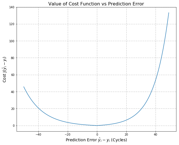
In our case, a good option suggested in the literature is the function J below:

$J = \begin{cases} \sum_{i=1}^{N}e^{-(\frac{\hat y_{i} - y_{i}}{13})} - 1,& \text{if } \hat y_{i} - y_{i} < 0 \\ \sum_{i=1}^{N}e^{(\frac{\hat y_{i} - y_{i}}{10})} - 1,& \text{if } \hat y_{i} - y_{i} \geq 0 \end{cases}$

Where N is the total number of engines under evaluation, and $\hat{y}_{i}$ and $y_{i}$ are the predicted and true values for the RUL of an engine i, respectively. As shown by the plot of J in the figure above, this function correctly penalizes overestimates ( $\hat{y}_{i}-y_{i}\geq0$ ) more than underestimates ( $\hat{y}_{i}-y_{i}<0$ ) of the true RUL, thereby capturing our intuition about the different penalties associated with each.

What’s next?

It’s easy to see that the data set described above represents a nice testbed for experimenting with and evaluating different approaches to the problem of predictive maintenance. In future posts, we’ll dive deeper into the dataset and illustrate some promising approaches to the RUL estimation problem.

Want to play with the data yourself? In this repository, you’ll find some scripts and a notebook to get you started.