
How to Navigate the Jupyter Ecosystem
For Data Science Teams | February 28th, 2017
Project Jupyter encompasses a wide range of tools (including Jupyter Notebooks, JupyterHub, and JupyterLab, among others) that make interactive data analysis a wonderful experience. However, the same tools that give power to individual data scientists can prove challenging to integrate in a team setting with additional requirements. Challenges stem from the need to peer review code, to perform quality assurance on the analysis itself, and to share the results with management or a client expecting a formal document.
In this post, we’ll be talking through a few tools that help make data science teams more productive.
Sharing conda environments
The open source scientific software stack has many different tools that are useful and justifiably popular. Conda is an environment manager that allows data science teams to share environments. An excellent analysis of conda (especially in comparison to virtualenv) can be found in Jake Vanderplas’ article Conda: Myths and Misconceptions.
Especially on data science teams that are installing their own packages, having a mismatch between versions of libraries can cause problems. Using conda to set up your environments, and further taking advantage of anaconda.org to host the conda environment, lets the data science team share the environment with a few simple commands (for example):
(Assuming you already have conda installed and are using bash shell.)
    envname='svdspy3'
    # to upload environments to anaconda.org only need to do once
    conda install anaconda-client conda-build
    # to update your conda to the most recent version
    conda install conda
    # Also update anaconda if you use that
    conda create --name $envname python=3 notebook pip matplotlib pandas jupyterlab
    pip install nbdime
    # Uncomment the next 2 `conda` lines if you want to upload
    # to anaconda.org (you will need to create username)
    # conda env export -n $envname > environment.yml
    # conda env upload $envname
Now for the useful part: anyone can now pull down this environment into their own workstation (in general):
    conda install anaconda-client conda-build
    conda env create $username/$envname
If you want to see this in action for yourself, you can run the following commands to get a reasonable starting conda environment for data science:
    conda env create qwpbqoiq/svdspy3
    # load it like any other conda environment
    source activate svdspy3
A couple of neat things to note about what just happened. First, the environment has a couple of surprising aspects: it contains packages that were pip installed, not conda installed. Second, besides the notebook, it also installed JupyterLab, which is currently an alpha-stage app within the Jupyter project. It combines the Notebook with an environment that allows for greater much flexibility and integration. Doing this process to share a conda environment across a data science team can ease the friction of sharing results and work between team members.
Version control with Notebooks (nbdime)
Working in a data science team means sharing work with one another for many different stages: code review, peer review of techniques, collaboration on a single Notebook. It has long been somewhat painful to combine Notebooks and version control in a seamless fashion. The choices come down to one of two paths, each of which creates some friction. The first option is to strip out all output from a Notebook before committing, and committing with outputs (and the extra megabytes) to allow for easier peer review or quality assurance of results. If the plots under review require even a few minutes of data processing, then re-running “no-output” notebooks becomes a barrier to providing feedback across multiple teams.
Another common use case of Notebooks is to demonstrate how to use a new package, or how you solved a problem. Without embedding the output, you will only see the input code and you might end up with demonstration notebooks that show off your (probably) amazing new library that look completely blank. This notebook (and far too many like it) is supposed to show off what can be done with a new library or tool, but you have to use your imagination to guess what it does. Or you require people to clone your repo, install your library, and rerun your notebook to see the results. These are use cases where including output in the Notebooks might be a better idea.
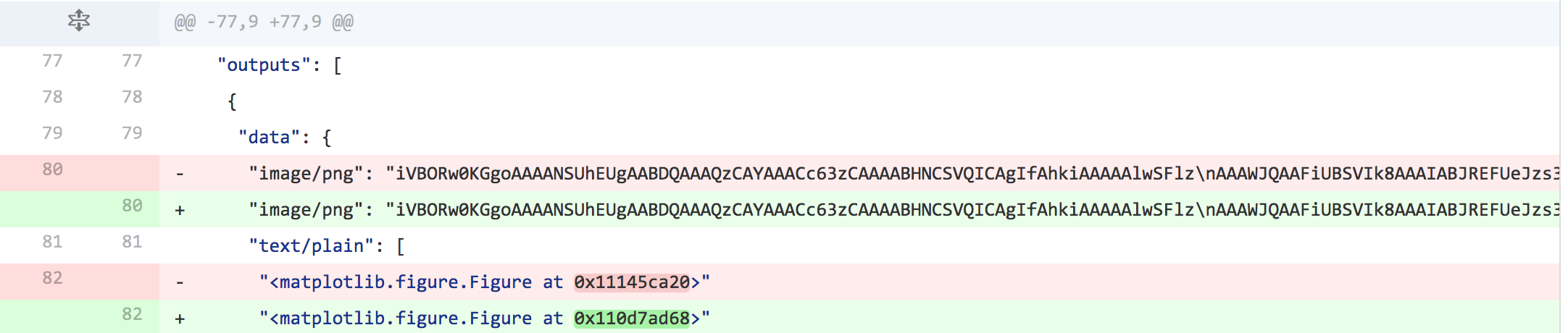
That brings us to the the other option: committing your Notebooks and including the output. The upside for this is approach is that reviewing the quality of a fit, by looking at the output, is dead simple when you have the plot included. It is also rendered natively on github these days. The downside is that version control tends to fight the output stored by a Notebook, and the current situation, if you update a plot, for example, you get a git diff that looks like this:
A tool has just been released (still early stages) that really helps with this situation: nbdime. Nbdime is a module that integrates a number of features that lets users much more easily do something data scientists have long clamored for: easy diffs of Notebooks.
Update a plot in a Notebook, git commit, and now the diff looks like (from the nbdime docs) this:
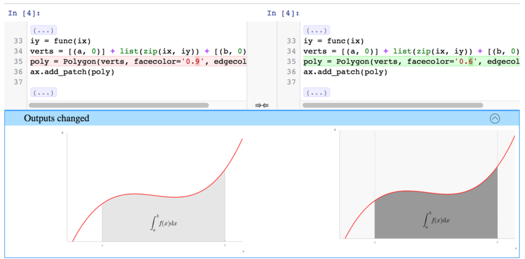
which shows the difference in the plot side-by-side.
This comparison is a huge improvement over the previous scenario—which would require saving the image as a png, committing this file, and using github’s internal tools to detect that the plot image has been updated, giving you a side-by-side look.
JupyterHub
As data science consultants, we have come across all manner of working situations, with varying degrees of freedom in how we as a team can jump into the client’s existing data science framework. Each team member logging in via their own laptop to a common edge node and sharing results from a git repository is a common setup. Another one that we are seeing more frequently (and encourage the use of) is an installation of JupyterHub on a client’s server.
JupyterHub is a central server that will run the backend for Jupyter Notebooks. Setting up JupyterHub is beyond the scope of this blog post, as there are many site-specific considerations to take into account. Here is a link JupyterHub’s documentation to help you set this up. JupyterHub is usually located on a cluster’s edge node, which means that the processing power (and RAM) of an edge node is the workhorse behind your analysis. Further, accessing data for analysis is usually much easier and faster when the server is located on the same cluster behind the firewall.
One advantage of running a common JupyterHub server: sharing and copying Notebooks between data scientists is easier when they are all on the same server. By default, JupyterHub users can only access directories in their home directories, but if people put a symbolic link in their home directories to a shared directory between all team members, then the team can see and run each other’s Notebooks. This moves the barrier to collaboration even lower.
For examples of how to organize the structure of that shared directory, you can see either Cookie Cutter Data Science, or reference some of our previous blog posts on Jupyter Notebook Best Practices.
Editor’s note: Jonathan (as well as other members of SVDS) spoke at TDWI Accelerate in Boston. Find more information, and sign up to receive our slides, here.
sign up for our newsletter to stay in touch