Getting Started with Predictive Maintenance Models

May 16th, 2017

In a previous post, we introduced an example of an IoT predictive maintenance problem. We framed the problem as one of estimating the remaining useful life (RUL) of in-service equipment, given some past operational history and historical run-to-failure data. Reading that post first will give you the best foundation for this one, as we are using the same data. Specifically, we’re working with sensor data from the NASA Turbofan Engine Degradation Simulation dataset.

In this post, we’ll start to develop an intuition for how to approach the RUL estimation problem. As with everything in data science, there are a number of dimensions to consider, such as the form of model to employ and how to evaluate different approaches. Here, we’ll address these sub-problems as we take the first steps in modeling RUL. If you’d like to follow along with the actual code behind the analysis, see the associated GitHub repo.

Benchmarking

Before any modeling, it’s important to decide how to compare the performance of different models. In the previous post, we introduced a cost function J that captures the penalty associated with a model’s incorrect predictions. We are also provided with a training set of full run-to-failure data for a number of engines and a test set with truncated engine data and their corresponding RUL values. With these in hand, it’s tempting to simply train our models with the training data and benchmark them by how well they perform against the test set.

The problem with this strategy is that optimizing a set of models against a static test set can result in overfitting to the test set. If that happens, the most successful approaches may not generalize well to new data. To get around this, we instead benchmark models according to their mean score over a repeated 10-fold cross validation procedure. Consequently, each cross validation fold may contain a different number of test set engines, if the training set size is not divisible by the number of folds. Since the definition of J from the previous post involves the sum across test instances (and thus depends on the test set size), we instead modify it to be the mean score across test instances.

The benchmarking will take place only on data from the training set, and the test set will be preserved as a holdout which can be used for final model validation. This procedure requires us to be able to generate realistic test instances from our training set. A straightforward method for doing this is described in this paper.

Information in the sensors

Most of the sensor readings change over the course of an engine’s lifetime, and appear to exhibit consistent patterns as the engine approaches failure. It stands to reason that these readings should contain useful information for predicting RUL. A natural first question is whether the readings carry enough information to allow us to distinguish between healthy and failing states. If they don’t, it’s unlikely that any model built with sensor data will be useful for our purposes.

One way of addressing this is to look at the distribution of sensor values in “healthy” engines, and compare it to a similar set of measurements when the engines are close to failure. In the documentation provided with the data, we are told that engines start in a healthy state and gradually progress to an “unhealthy” state before failure.

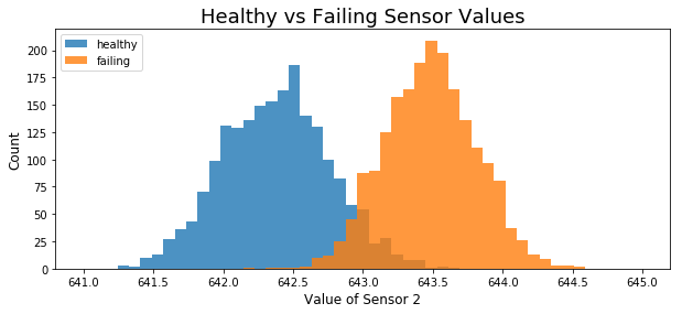
The figure above shows the distribution of the values of a particular sensor (sensor 2) for each engine in the training set, where healthy values (in blue) are those taken from the first 20 cycles of the engine’s lifetime and failing values are from the last 20 cycles. It’s apparent that these two distributions are quite different. This is promising—it means that, in principle, a model trained on sensor data should be able to distinguish between the very beginning and very end of an engine’s life.

Mapping sensor values to RUL

The above results are promising, but of course insufficient for the purposes of RUL prediction. In order to produce estimates, we must still determine a functional relationship between the sensor values and RUL. Specifically, we’ll start by investigating models () of the form described below, where is the RUL for engine j at time t, is the value of sensor i at that time.

(1)  

It’s important to note here that this isn’t the only way to estimate RUL with this kind of data. There are many other ways to frame the modeling task that don’t require a direct mapping from sensor values to RUL values at each time instant, such as similarity or health-index based approaches. There is also a whole class of physical models that incorporate knowledge about the physics of the underlying components of the system to estimate its degradation. To preserve generality and keep things simple in the discussion below, we won’t consider these approaches for the moment.

Linear regression

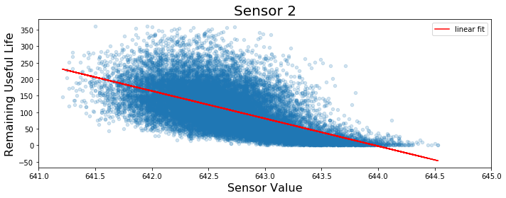
A simple first approach is to model as a linear combination of ’s:

(2)  

This is illustrated in the figure below. In blue are the values of a particular sensor (sensor 2 in this case) plotted against the true RUL value at each time cycle for the engines in the training set. Shown in red is the best fit line to this data (with slope ).

The figure below shows the performance of the linear regression model (using all sensor values as features). Each point represents a single prediction made by the model on a test engine in the cross validation procedure. The diagonal line represents a perfect prediction (). The further a point is away from the diagonal, the higher its associated cost.

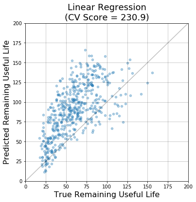
Given the plots above, there are a few reasons to think this approach is perhaps too simple. For example, it is clear that the relationship between the sensor values and RUL isn’t really linear. Also, the model appears to be systematically overestimating the RUL for the majority of test engines. Using the same inputs, it’s reasonable to think that a more flexible model should be able to better capture the complex relationship between sensor values and RUL.

More complex models

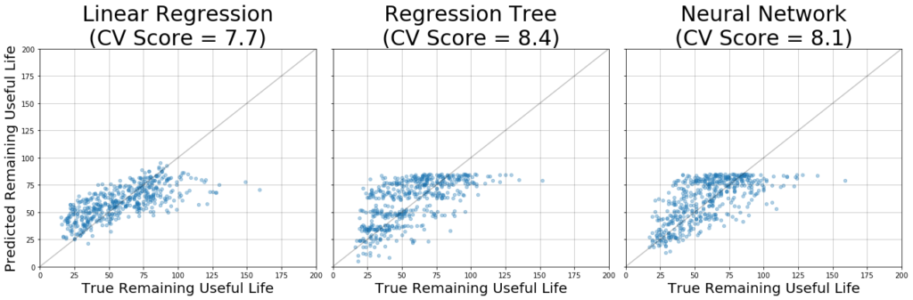
For the reasons just mentioned, the approach above is likely to be leaving a lot on the table. To evaluate this idea, two other models were trained on the same task: a regression tree and a feedforward neural network. In both cases, hyperparameters were optimized via cross validation (not shown), resulting in a tree with a maximum depth of 100 and neural network with two 10-unit hidden layers. The figure below shows diagnostic plots of these models, along with their scores.

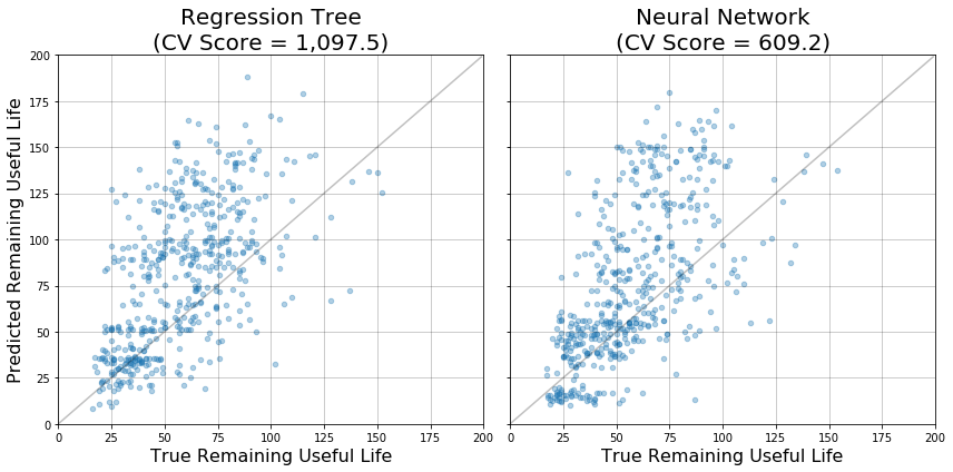
Notice that in both cases, the models appear to capture some characteristics of the expected output reasonably well. In particular, when the true RUL value is small (~25 to 50) they exhibit a high density of predictions close to the diagonal. However, both of these models score worse than the simpler linear regression model (higher CV score).

To get a feel for exactly how these models are failing, recall that our cost function scales exponentially with the difference between predicted and true RUL, and overestimates are penalized more heavily than underestimates. In the figure above, this difference corresponds to the distance along the y-axis from each point to the diagonal. Notice that when the true RUL is in the range of about 50 to 100, both models tend to overestimate the RUL by a lot, leading to poor performance.

Improving the models

To understand how to improve our models, it’s necessary to take a step back and examine exactly what we are asking them to do. The figure below shows some example sensors from an engine in the test set plotted over time. The dashed line shows the corresponding RUL at each time step which, as we’ve (implicitly) defined it, is linearly decreasing throughout the life of the engine, ending at 0 when the engine finally fails.

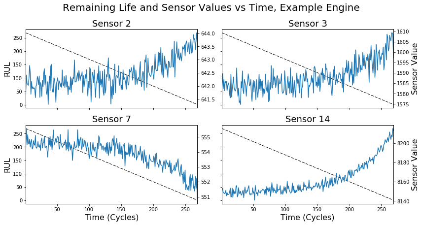
Notice that only near the end of the engine’s life do the sensor readings appear to deviate from their initial values. At the beginning (about cycles 0 through 150 in the figure above), the sensor readings are not changing very much, except for random fluctuations due to noise. Intuitively, this makes sense—even though the RUL is constantly ticking down, a normally-operating engine should have steady sensor readings.

Given how we’ve framed the predictive modeling task, this suggests a major problem. For a large portion of each engine’s life, we’re attempting to predict a varying output (RUL), given more or less constant sensor values as input. What’s more, reliably predicting RUL values of healthy engine cycles won’t necessarily guarantee better performance on the test set¹. As a result, these early engine cycles are likely contributing a large amount of training set error, the minimization of which is irrelevant to performance on the test set.

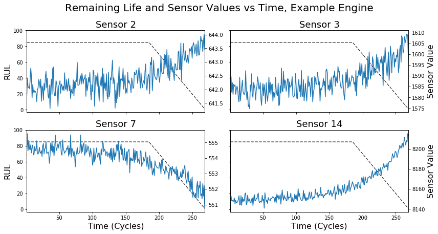
One approach to this issue is illustrated by the dotted line in the figure above, in which we redefine RUL. Instead of assigning an arbitrarily large RUL value across the life of the engine, we can imagine limiting it to a particular maximum value (85 in this case). If RUL is related to underlying engine health, then this is intuitive: the entire time an engine is healthy, it might make sense to think of it as having a constant RUL. Only when an engine begins to fail (some set amount of time before the end of its life) should its declining health be reflected in the RUL.

The models described above were re-trained using this modified RUL assignment scheme (max RUL = 85), and results are shown in the figure above. Notice that this simple tweak yields an order of magnitude gain in performance across all models, as measured by the overall cost. From the figure it’s apparent that this alternative labeling results in an upper limit on the RUL predictions that the model can make, which makes sense given the inputs. As a result, these models are less prone to the drastic overestimates that plagued the previous versions.

There are still many aspects of this problem still left to explore. From the figures above, it’s clear that the models struggle to produce accurate estimates when the RUL is especially large or small. Also, we’re treating each time point as an independent observation, which isn’t quite right given what we know about the data. As a result, none of our models take advantage of the sequential nature of the inputs. Additionally, we aren’t doing any real preprocessing or feature extraction. Nevertheless, compared to our initial models, we’ve managed to demonstrate a significant improvement in predicting RUL.

What’s next?

In future posts, we’ll dig a bit deeper into some of the nuances of this problem and develop a better intuition for approaching predictive maintenance in IoT systems. Want to play with the data yourself? In this repository, you’ll find some scripts and notebooks to get you started.

sign up for our newsletter to stay in touch

Bottom: ^{1. Recall that the challenge is to predict a single RUL value after observing a series of sensor measurements. A quick look at the test set shows that many of the true RUL values are in the range of 25 to 100, presumably when these engines are no longer healthy.↩}